Medical physics with Geant4 + Docker = ❤️

In this lab we will learn about the basics of low and mid-energy radiation-matter interaction with the help of Geant4, the Geant4 binding for Python (g4py), and of course, our beloved Docker. This lab may fall into the recent (and praiseworthy) trend related to the so called reproducible research and Open Educational Resources as a Service. This PWD/Docker-based experience has been carried out with huge success at Universidad Internacional de La Rioja (UNIR), as described in this research paper.
Simulating the building blocks of Reality
To begin with, let’s start by summarising what is Geant4 and why it is so important in todays particle physics research. As very well stated by Agostinelli et al.:
Geant4 is a toolkit for simulating the passage of particles through matter. Its functionalities include tracking, geometry, physics models and hits. The physics processes take into account electromagnetic, hadronic and optical processes, as well as the surrounding materials, over a wide energy range. The toolkit is the result of a worldwide collaboration of physicists and software engineers. It has been implemented in the C++ programming language. It has been used in applications in Particle Physics, Nuclear Physics, accelerator design, Space Engineering and Medical Physics.
 In other words, Geant4 implements our deepest (and best) level of knowledge about Nature… in the form of computer (C++) code. This deepest level is no other thing but the Standard Model of physics. This picture describes the building blocks of Reality (the subatomic particles) as well as the fundamental forces that govern their interactions. Geant4 acts as some sort of magnifying lens that amplifies what happens when a given particle (an electron, a kaon, a muon, or a photon) hits or, better said, interacts with its surroundings. This computer toolbox is able to simulate almost all possible scenarios, no matter the actors involved, the geometry or the energy of the event.
This turns out perfect if we happen to be particle physicists, but it may be felt as over complicated for those who just need to model humbler atomic interactions for specific fields. One if these specific fields is Medical Physics and, in this case, Geant4 has a wonderful and easy to use Python binding, g4py. With the help of Docker, g4py is even easier to use.
Particle Physics in Medicine
The field of Medical Physics has its own complexity. Subatomic particles can be used to treat cancer or tumours or can be used to image (probe) a patient’s body, i.e., to see its inner parts. This last application is the one that will be tackled in this interactive lab. Normally, the type of imaging particle will be the (X-ray) photon, although you’ll be able to play with other probing rays such as electrons or positrons. Photons can be defined as particles of light and were originally proposed by Einstein in one of his 1905 paper An Heuristic Point of View Toward the Emission and Transformation of Light.
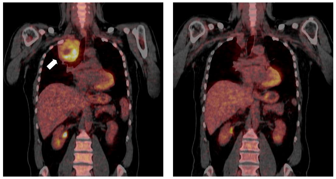
In Medical Imaging, mid-energy photons (a few keV) are projected against the patient. Some of these electromagnetic entities are completely absorbed (photoelectric effect), others are diverted (Compton scattering) by atoms, and others (if their energy is high enough) can even transform themselves into a pair of new objects composed of a electron and an anti-electron (a positron). This last process is called pair production. In turn, when a positron accidentally hits and electron, they both disappear back into two photons which travel in opposite directions. This is called annihilation and it’s the foundation of PET imaging (which produces beautiful and lifesaving images such as the one shown above).
Geant4 and Medical Physics
 As stated above, Geant4 has a difficult-to-grasp C++ heart, but thanks to g4py, its easy to design simple scenarios related to the field of Medical Physics which radiologists and doctors can even used in their daily practice. However, installing and configuring Geant4 and g4py can turn out awkward. We can alleviate this problem with Docker and better yet, we can play with a simple, yet interesting simulation thanks to Play with Docker. This simulation consists of the following ingredients:
- A world, or the simulation limits. This world has the shape of an empty elongated cuboid. The longest axis is the
z(or longitudinal) axis. - A beam of particles that are initially projected along the aforementioned
z-axis. This beam has a nature (type of particles), an energy (in mega-electronvolts or MeV, for short) and a count (i.e., how many particles). In a real particle physics experiment or setup, generating (and conforming) such a beam has its complexities. However, in a simulated world, we don’t have to worry about those. - A target, or something the particles can hit in their way. This target has also cuboid shape, with a width (thickness) and location (both also defined along the same
z-axis as the world) and is composed of a given (and selectable) material. In Medical Physics, the target is also commonly known as phantom.
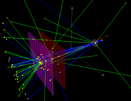
You can take a 3D look at this world in the following image:

Or you can also surf a live WebGL version by clicking in this link. A quick (and tiny) animation is also displayed above.
We will now launch our own simulations. In order to achieve so, let us first download the Docker image that contains the necessary infrastructure. Remember, you can just click in the code cells to have them (one by one) executed ▶️ in the terminal on the left side of this page:
docker pull pammacdotnet/g4lpwd
It may take a minute 🕐 or so to download the whole image… so please, be (slightly) patient.
Download the simulation code from Github
The code of the simple simulation described above can be downloaded by clicking in the next code cell:
curl https://raw.githubusercontent.com/pammacdotnet/FFRepo/master/simulation.py -o simulation.py -s
We recommend you take a quick look (even if you are not a Python or particle physics enthusiast) so that you realise how it is very easy to experiment with modern computer simulations thanks to awesome tools such as g4py:
pip install pygments
pygmentize -g simulation.py
Also, download (and enable the execution of) this simple Python script to convert from WRL data to x3dom-enabled HTML content:
curl https://raw.githubusercontent.com/pammacdotnet/FFRepo/master/wrl2html.py -o wrl2html.py -s
chmod +x wrl2html.py
This will allow us to visualise 3D scenes (like the one linked above) in the same Web browser. BTW, this last command (wrl2html.py) uses this online converter made by the company instantreality (part of the Visual Computing System Technologies Group which, in turn, belongs to the reputed Fraunhofer Institute).
First simulation
Let’s run our first simulation. It will consist of a beam of 20 photons, each of 1 MeV that hits a water filled target (with a thickness of 20 cm):
docker run -v ${PWD}:/root pammacdotnet/g4lpwd
You’ll see a bunch of information appearing in the terminal:
**************************************************************
 Geant4 version Name: geant4-10-04-patch-02    (25-May-2018)
                       Copyright : Geant4 Collaboration
                      References : NIM A 506 (2003), 250-303
                                 : IEEE-TNS 53 (2006), 270-278
                                 : NIM A 835 (2016), 186-225
                             WWW : http://geant4.org/
**************************************************************

Visualization Manager instantiating with verbosity "warnings (3)"...
/tracking/storeTrajectory 1
/tracking/storeTrajectory 2

phot:   for  gamma    SubType= 12  BuildTable= 0
      LambdaPrime table from 200 keV to 100 TeV in 61 bins
      ===== EM models for the G4Region  DefaultRegionForTheWorld ======
       PhotoElectric :  Emin=        0 eV    Emax=      100 TeV   AngularGenSauterGavrila

compt:   for  gamma    SubType= 13  BuildTable= 1
      Lambda table from 100 eV  to 1 MeV, 7 bins per decade, spline: 1
      LambdaPrime table from 1 MeV to 100 TeV in 56 bins
      ===== EM models for the G4Region  DefaultRegionForTheWorld ======
…
…
This is Geant4 telling you all the calculations it has had to carry out for you in behind the scenes in order to generate a final (and more intuitive) file called simulation.wrl (default name). It is now time to launch a simple web server that will let us download or view the results:
python3 -m http.server 80 > /dev/null 2>&1 &
By using the & symbol we state we want the web server to run in the background and with the expression > /dev/null 2>&1 we guarantee that its output won’t bother us. Once started, the previous file can be downloaded from here ⬇️. It’ll take some time because a VRLM file can be quite big.
Once in your hard drive, you can 3D-navigate/fly through this file (or any VRML scene) with any of the following software:
- Instant Player, by instantreality,
- view3dscene, by Castle Game Engine,
- Paraview, by Kitware and,
- Blender (among many others).
Here you can see a screenshot of view3dscene (Windows version):

However, it is better to transform the WRL file into WebGL-enabled HTML with the wrl2html.py command tackled above:
./wrl2html.py
By default, this last command assumes the input WRL file to have the name simulation.wrl and outputs an HTML file called, by default, simulation.html. You previous instruction is equivalent to:
./wrl2html.py --wrl simulation.wrl --html simulation.html
You can fly through this 3D HTML version by clicking here ↗️, or you can list all files 📁.
More simulations
Let’s explore more simulations! You achieve this by altering any of the configurable parameters:
- Particle type. Available with the option
--type. Possible values aree-,e+orgamma. The default value isgamma(also known as photons or, simply, light). - Particle energy. Available with the option
--energy. All values are expressed in MeV and should be integer values. The default values is 1 (MeV). Bear in mind that X-rays have more or less 0.1 MeV of energy. - Phantom material. Available with the option
--material. Geant4 defines many materials:G4_Al,G4_Si,G4_Ar,G4_Cu,G4_Fe,G4_Ge,G4_Ag,G4_W,G4_Au,G4_Pb,G4_AIR,G4_Galactic,G4_WATER,G4_CESIUM_IODIDE,G4_SODIUM_IODIDE,G4_PLASTIC_SC_VINYLTOLUENE,G4_MYLAR, etc. The default value in our simulations is water (G4_WATER). Do you remember that the human body is composed of 70% water? - Phantom thickness. Available with the option
--size. It is the size (along the longitudinal axis) of the phantom, that is, how much matter the beam of particle will have to traverse. - Output file. Available with the option
--wrl. It represents the name of the VRML file with a 3D representation of the simulation. The default value issimulation.wrl. - Particle count. Available with the option
--count. It is the number of particles within the simulated beam. The default value is 20. We suggest that you keep this value under 💯. Otherwise you’ll end up with a huge WRL file, very difficult to manage and visually analyse.
Antimatter to the rescue!
For instance, the following command:
docker run -v ${PWD}:/root pammacdotnet/g4lpwd --type=e+
will exchange photons for positrons. Positrons are the antiparticles of electrons. The major difference from electrons is their positive charge. You can either download again the WRL file ⬇️ or generate a new HTML file. If you run again the wrl2html.py command with no arguments, the original simulation.html file will be overwritten ⚠️. However you can change the name of the resulting HTML file:
./wrl2html.py --html simulation2.html
This file is still browsable ↗️.
 Positrons tend to annihilate with electrons. When this happens, two photons emerge in opposite directions. As you can see from the following picture, the positrons (yellow traces) suddenly seem to disappear. What is happening is that those positrons find a corresponding electron (attached to the atoms that compose the material) and the mass of both particles is transformed into two photons emerging in any random direction (but opposite ways).

Light seems to zigzag!
 Another effect that you will see in the previous simulation is that light rays seem to bend with sharp angles. This is due to the Compton scattering. In this process, the path of a photon is diverted by a charged particle, usually an electron. In each scattering event, the ray of light loses energy (decreases its frequency) and its finally absorbed by the material.

Superman (o Supergirl)-approved shielding!
Let’s now change the particle type to a more common one (electrons) and let’s have them collide against a lead target:
docker run -v ${PWD}:/root pammacdotnet/g4lpwd --type=e- --material=G4_Pb --wrl simulation3.wrl
./wrl2html.py --wrl simulation3.wrl --html simulation3.html
The results are displayed here ↗️. Again, you can specify a new WRL file (with the --wrl option). As you can see, 1 MeV electrons are unable to penetrate the material. On the contrary, some of them seem to bounce back. This is due to electrostatic repulsion against the electronic cloud covering this lead shield.

Beware of radiation!
Let’s repeat the same simulation with a (virtual) water target and with a greater energy:
docker run -v ${PWD}:/root pammacdotnet/g4lpwd --type=e- --energy=100 --wrl simulation4.wrl
./wrl2html.py --wrl simulation4.wrl --html simulation4.html
 If you carefully observe the simulation results ↗️, you’ll notice the famous electromagnetic showers. This is the same process that occurs when a cosmic ray hits the upper atmosphere and triggers the generation of new particles. The primary process that we are watching here is bremsstrahlung, which consists in the production of electromagnetic radiation (a photon, represented by a white line) when an electron decelerates by the presence of matter.

Remember you can either download the resulting WRL file or navigate through the x3dom-enabled HTML file.
Ionization
Many of the already proposed simulations exhibit ionisations. In this type of interaction, a photon hits an electron (attached to an atom) and produces an ion (i.e., an atom negatively charged).

The previous simulation was obtained with the following command (and whose results can be explored here ↗️):
docker run -v ${PWD}:/root pammacdotnet/g4lpwd --type=gamma --energy=10 --material=G4_Al --wrl simulation5.wrl
./wrl2html.py --wrl simulation5.wrl --html simulation5.html
Ionisations can also take place when a moving electron hits an atom at rest (well, one of its orbiting electrons), that is, the ionisation particle can be of the same nature as the removed one.
Simulation limits and photoelectric absorption
Let’s go back a water-filled cuboid and low energies, but let’s insanely increase the number of particles (photons). Run the following command in the terminal:
docker run -v ${PWD}:/root pammacdotnet/g4lpwd --type=gamma --energy=2 --count=100 --wrl simulation6.wrl
./wrl2html.py --wrl simulation6.wrl --html simulation6.html
You’ll see an scenario ↗️ very similar to this one, where the photons, after traveling in straight lines and/or interacting with matter, seem to disappear:

Well, where did all the photons go? Well, some of them reach the world limits… Do you remember the movie The 13th Floor?
Here you have a second simulation that better shows the previous processes:

This scene can be recreated with the following command, where a beam of just a few electrons hits an iron target:
docker run -v ${PWD}:/root pammacdotnet/g4lpwd --type=e- --material=G4_Fe --count=10 --energy=50 --wrl simulation7.wrl
./wrl2html.py --wrl simulation7.wrl --html simulation7.html
Each electron produces in turn an electromagnetic shower. These showers consist of a bunch of photons that end up photoelectrically absorbed. Take a look ↗️ for yourself (of course, after running the simulation)!
Energy is a kind of matter
 Yes, energy can be transformed into matter (and back!)… as discovered by Einstein in his famous 1905 paper: On the Electrodynamics of Moving Bodies. BTW, Einstein was also responsible for the explanation of the photoelectric effect, as commented in the introduction above.
(Not that Einstein!)
Run the following simulation:
docker run -v ${PWD}:/root pammacdotnet/g4lpwd --type=gamma --material=G4_WATER --count=10 --energy=15 --wrl simulation8.wrl
./wrl2html.py --wrl simulation8.wrl --html simulation8.html
You will see ↗️ some events like the following, where a photon (with no mass and thus made of pure energy), after colliding with an atom, transfers all its momentum to the creation of two particles: an electron and anti-electron (positron). 
That is: energy (E) is eventually converted into matter (m), following the famous Einstein equation: E=m·c·c, where c is the speed of light. This process is known as pair production.
Final words
Now it’s time for you to play with your own simulations. This includes other materials, energies, particles, etc. As stated above, you can also increase the number of particles, but we suggest you keep this number below 100. This lab is based on the article X-ray imaging virtual online laboratory for engineering undergraduates (by Alberto Corbi, Daniel Burgos, Frank Vidal, Francisco Albiol and Alberto Albiol) and it has been carried out with success in the first semesters of the Computing Science degree at the School of Engineering of Universidad Internacional de La Rioja (UNIR).


